Pan/Tilt Motion System for Control Education

Ricardo G. Sanfelice, University of Arizona

Project supported by Mathworks

Website developed by Colin Lasharr, University of Arizona

Introduction

The device is composed of a rotating base with an elevation arm to orient the attitude of energy collectors, which are modular. The base of the device is linked to a drive train that is powered by a small servo motor and provides the propulsion to orient the attitude of the device. The elevation arm is connected to another small servo motor which provides the propulsion to orient the altitude of the device.

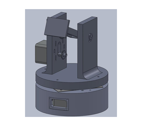
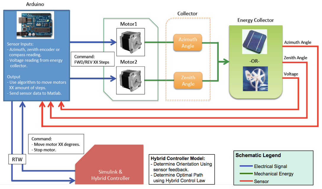
The system is composed of an Arduino control board that receives input from the Simulink controller in real time, and then sends output to the motors. There are two stepper motors which control the zenith and the azimuth angles. These motors position the base and arm of the device.

Instructions for Building the System

Installation Instructions

The device is powered by a USB port. It communicates with MATLAB through a generic USB to Serial driver which comes with Windows operating system. At this time, the target board operates on Win32 platforms only. It has been tested with MATLAB Release 2011a. The installation process includes the following steps:

Plug in the Arduino USB into the desktop to recognize the new hardware.
Go to Start -> Control panel -> System -> Hardware -> Devicemanager -> Ports(COM & LPT), to recognize the new hardware communication port.
Install the Arduino supporting drivers from the following link:http://arduino.cc/en/Guide/Windows#toc4
Setup the device with the drives following the instructions on the following page:http://arduino.cc/en/Guide/UnoDriversWindowsXP
Install the Arduino, Matlab supporting files to initialize the controller board from the following link: http://www.mathworks.com/matlabcentral/fileexchange/32374
Make sure the files associated with the current model are pointed towards the Matlab files downloaded in the previous step.
Execute the following initialization files: arduino.m and install arduino.m (from the downloaded matlab folder ArduinoIO -> simulink)
Run the model with desired inputs

The Arduino Board

The Arduino Motor Shield can easily interface with a host PC through Simulink with the Arduino IO package provided by Mathworks. The Arduino IO package allows for any blocks developed in Simulink to quickly interface with an ATMega328 running an Arduino IO server on the Arduino Boot Loader. With the use of the Real-Time Pacer block to match the simulation clock to real time, models can run in real time with the physical system.

Simulink

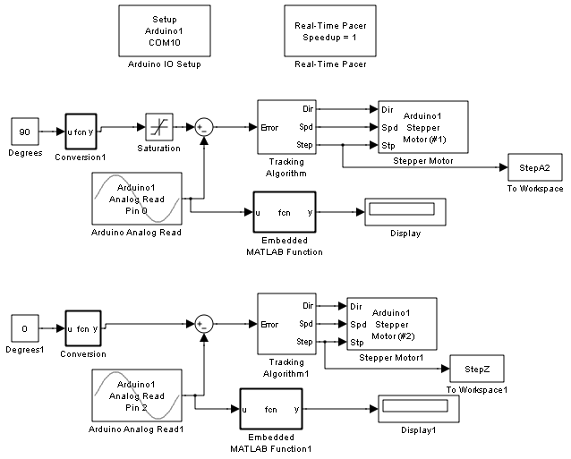
This simple block diagram provides real time communication between the board and Simulink. The control algorithm controls one of the degrees of freedom of the collector, and performs the same result for the second degree of freedom in the lower half of the diagram. Thus, we are able to perform the implementation of the control system through Matlab/Simulink. The interface for the integration of control designs created in Simulink are made fast and simple. They enable students to implement their control algorithms from their class in a very efficient and quick manner.

The dynamics of the closed-loop system, including actuators, plant, and sensors, are modeled mathematically using circuitry, rigid body, and aerodynamic principles. In most of the courses, the pan/tilt motion system is available to the student towards the end of the course, but preliminary modeling and control is done in related exercises throughout the course. Assignments are prepared requesting them to simulate their control designs. Using the SimMechanics toolbox, a model is created to simulate the equations of motion of the collector. This toolbox provides blocksets to simulate the bodies and joints that comprise the collector and is very useful when designing the control system to be implemented.

Initial Parameter Identification

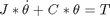
The zenith component of the pan/tilt motion system controls the solar panel arm of the device. This is the pitch component of the device and is powered by a simple stepper motor.

where J is the inertia of the rotor and load, C is the viscous damping coefficient, T is the load torque, theta is the angle, m is the mass of the arm, g is gravity and l is the length of the arm.

The azimuth component of the pan/tilt motion system controls the rotation of the base of the device. It is controlled by a simple stepper motor similar to the zenith component. The system is different due to the equations of motion being significantly different than the zenith component of the device.

where J is the inertia of the rotor and load, C is the viscous damping, theta is the angle, and T is the load torque.

System Identification for Zenith Component

Various controllers will be analyzed for the zenith control of the system including P, PI, PD, and PID control. After analyzing each of the controllers it is clear that a PID controller will counter the instability of the I control with the lag control of the D. This system should be tuned in order to reduce rise time and overshoot.

The system can analyzed using MATLAB’s system identification toolbox. The data is parsed into two separate signals. The input is labeled as u1 while the output as y1.

Note the slight time delay in the response. Using the system identification toolbox, the delay will be accounted for in the final model. Selecting both first order model and delay in the system identification toolbox, results in a simple transfer function that fits the system data.

The best fit estimation yielded a 99.52% match to the actual system which is accurate enough for the purposes of control. The transfer function takes the following form:

The values of Kp, Tp, and TD were given via the system identification toolbox (Matlab command: ident) such that the transfer function results as:

With this transfer function for the zenith angle, a root locus plot is generated to design a feedback controller. Since MATLAB does not support exponential terms in the transfer functions used in the root command, a Pade approximation is used. The Pade approximation is calculated using MATLAB’s pade command with a second order estimation (Matlab command: pade(G,2)). The pade estimation found was:

Multiplying P(s) by G(s) will yield the final transfer function for use in MATLAB’s root locus plot. To further verify that the estimation is accurate the approximation can be given a step input and the reaction can be measured (Matlab command: step(sys)). This can be compared to the system identification’s step function that was given.

System Identification for Azimuth Component

Similar to the zenith component, a model of the transfer function from input to azimuth angle is determined using the system identification toolbox in MATLAB. The proposed transfer function takes the form

Using the values provided by the system identification toolbox (Matlab command: ident), the resulting transfer function is

Again, a Pade estimation must be used to estimate the exponential for use with the root locus function in MATLAB. Using the pade estimation with a second order guess (Matlab command: pade(G,2)) gives

To ensure validity of the estimation the system identification step response can be compared to the estimated step response.

Even though the transfer function are different between the azimuth and zenith components the root locus plot takes a very similar shape. This is expected since the azimuth and zenith component use the same stepper motor and related hardware. The difference in the transfer function emerge from the distinct differences in the equations of motion of the two systems due to the moment arm of the zenith component.

As with the zenith angle many controllers were tested with a PID controller being selected due to the stability. The gains of the integral and derivative terms of the controller help reduce the rise time and overshoot.

Running An Experiment

To run a simple experiment in which the base and the arm both move to a specified angle, set the Degrees boxes to the desired angle, which will cause the base and the arm of the device to move that many degrees. To view the data from the variables, add a "To Workspace" block to each variable in order to receive the tracking and error data. Next, we run several experiments using different reference angles. The main Simulink file is available here.

Tracking and Error Data

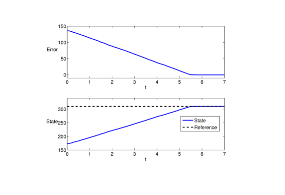
Error and trajectory plots for the azimuth angle (labeled as "state") (Matlab command: plot(data), hold on, and subplot). The target azimuth angle (labeled "Reference") is equal to 310 degrees. The intial angle is 175 degrees. The azimuth angle approaches the reference angle at around 5.5 seconds.

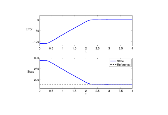
Error and trajectory plots for the zenith angle (labeled as "state"). The target zenith angle (labeled "Reference") is equal to 180 degrees. The intial angle is 290 degrees. The azimuth angle approaches the reference angle at around 2.2 seconds.

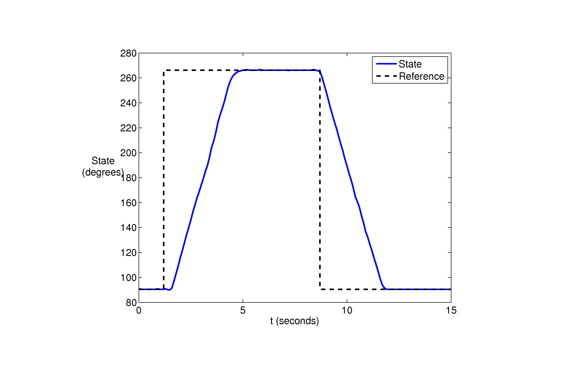
Response for tracking a step signal for the azimuth angle (labeled as "state"). The initial angle is 90 degrees and the target is 270. The step size is around 10 seconds. The azimuth angle converges to the target angle approximately 3 seconds after the reference angle changes value.

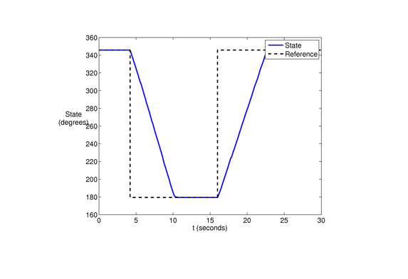
Response for tracking a step signal for the zenith angle. The initial zenith angle is 345 degrees with a step size of around 17 seconds. The target angle is 180 degrees. The trajectory converges to the target angle in approximately 6 seconds after the reference angle changes value.

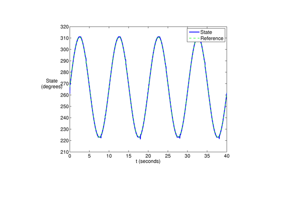
Tracking a sinusoidal reference input oscillating 45 degrees from a center 270 degrees azimuth angle, with a period of 10 seconds.

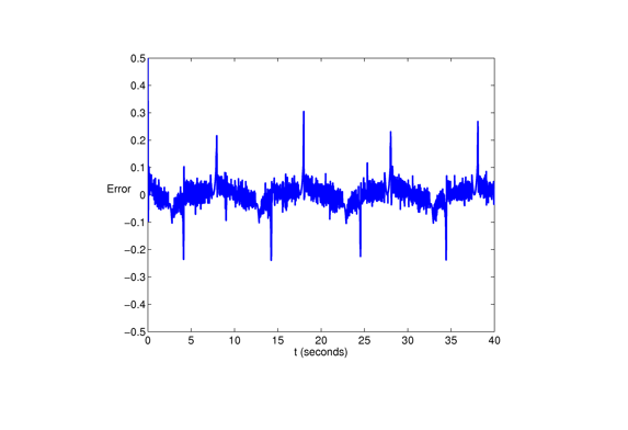
Tracking error for azimuth angle.

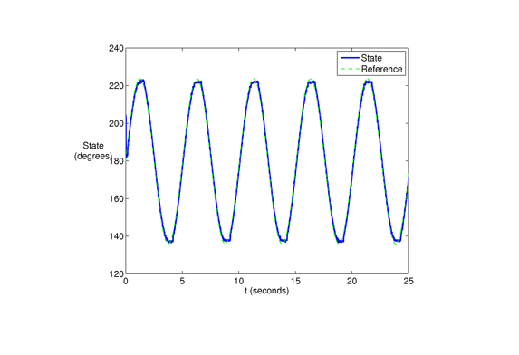
Tracking a sinusoidal reference input oscillating 45 degrees between 180 degrees for the zenith angle with a period of 5 seconds. The amplitude of the graph is approximately 45 degrees and the frequency will be approximately .2 oscillations per second.

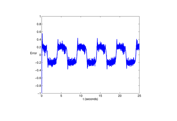
Tracking error for zenith angle.

Resources:

Summary of mechanical design and parts for the Pan/Tilt Motion System (for building).

Slides introducing the Pan/Tilt Motion Control System

Student reports from using in AME455, AME427, AME549 are available upon request.

Pan/Tilt Motion System for Control Education